This post is a follow-up to Basic causal inference via string diagrams. I apply the diagrammatic method outlined there to a (not so) simple problem of causal identifiability.
Diagrammatic causal inference (contd) : the new napkin problem
In The Book of Why, Judea Pearl gives an example of a causal effect that cannot be identified using either the frontdoor or the backdoor criteria, but requires the do-calculus to estimate. The problem is called the new napkin problem, in reference to an earlier problem that Pearl had solved on a napkin using the do-calculus.
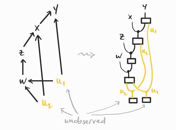
The effect to estimate is in the following causal model, which I draw below as a dag and as a string diagram, following the translation explained in the previous post:
Unfortunately, this time I do not have a story to motivate the model, nor does The Book of Why give one. The authors also leave open the question of whether can be identified, that is, expressed in terms of purely observational data.
It turns out that is identifiable and, in this follow-up post, I would like to re-derive the expression for , without using the do-calculus. I could not find a purely probabilistic argument anywhere, so I'm hoping this second post helps those who would like to see a derivation using only the usual rules of probability theory (and it was a nice exercise in causal inference). The proof below makes use of string diagrams, but these diagrammatic proofs are easy to translate to standard probabilistic notation. The diagrams are helpful visual guides that allow us to work both with the probabilistic data and the causal flow of information at the same time.
A short do-calculus derivation of can be found in this stackexchange answer by Carlos Cinelli. Their proof uses the backdoor adjustment formula as a lemma, albeit in a more general form than the one I gave in the previous post. This more general backdoor formula can also be derived in a few lines of do-calculus, but I will now derive it without it, in a few lines of diagrammatic calculus!
Backdoor adjustment revisited
In the previous post, I gave a rather simplified account of the backdoor adjustment, because I assumed that all variables were observed. In fact, it is obvious that, when there are no latent variables, all causal effects can be estimated from observational data. However, the backdoor formula also comes up in situations where there are unobserved variables. Let me explain this more interesting case via the same smoking example.
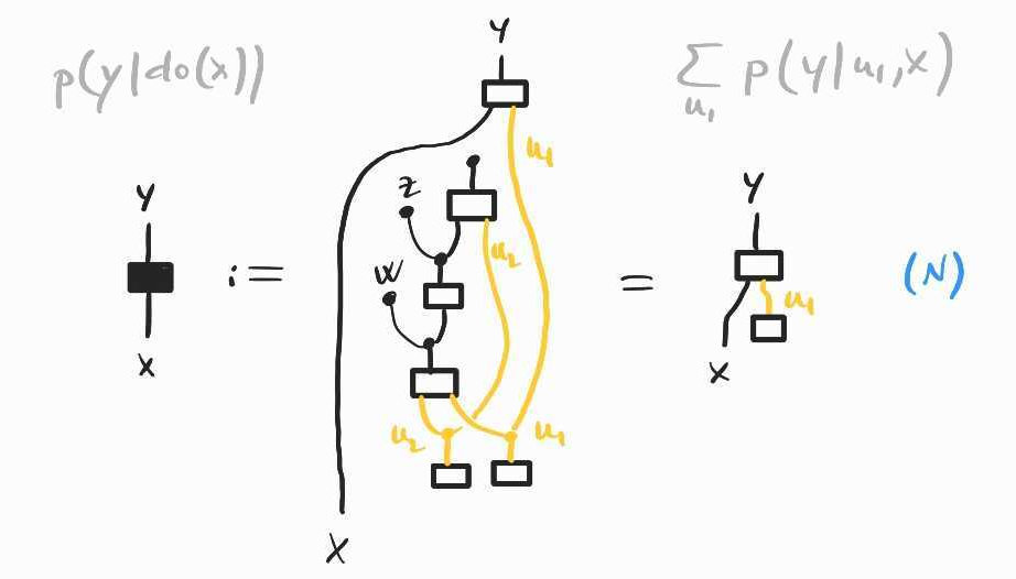
Going back to the smoking model of the previous post, suppose that we now want to estimate the causal effect of tar deposits in the lungs on cancer. That is, rather than , for which we developed the frontdoor formula, we want to estimate in the same causal model, which we reproduce below:
Once again, the interventional probability is not simply the conditional because of confounding factors, namely the hidden common cause , now mediated by . This can be seen in the following diagram for , which we obtain following the same approach as in the previous post:
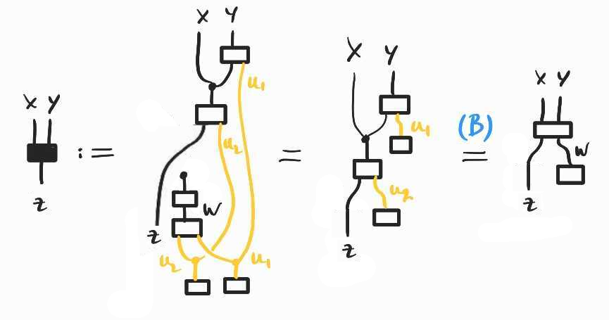
To identify , we need to rewrite this diagram in a form that does not contain the unobserved . To do this, we adopt a similar strategy as when we derived the frontdoor adjustment formula: we want to find a (set of) variable(s) such that and . The most probable candidate is , which turns out to work!
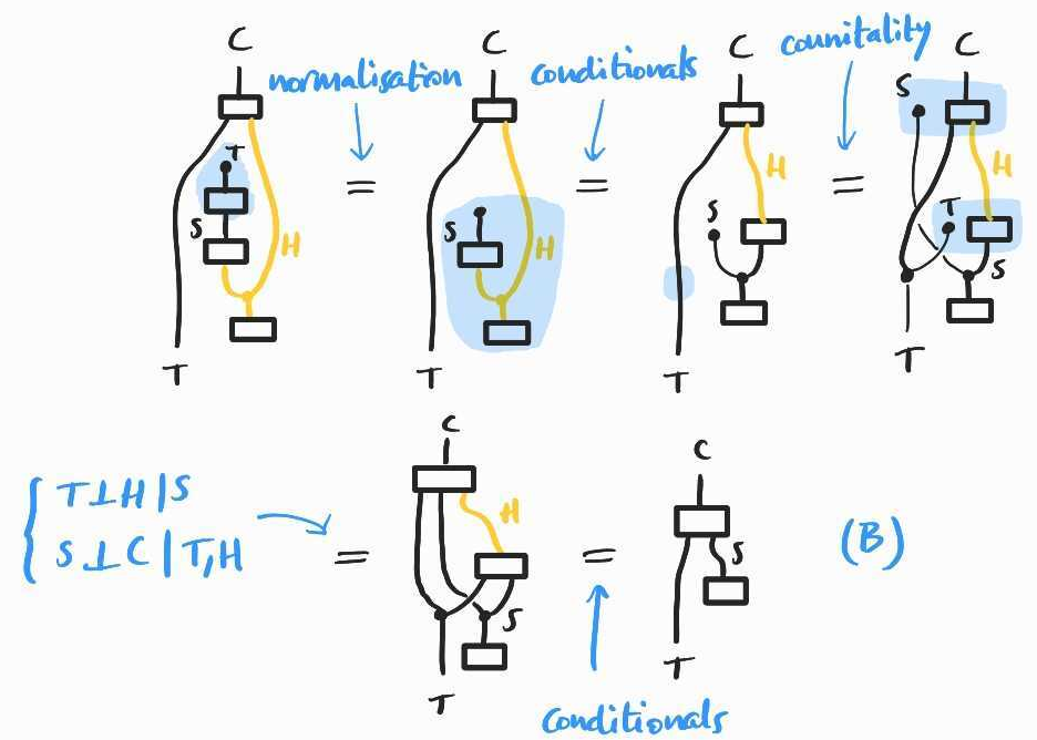
In probabilistic notation, we have shown that –a formula that we call (B).
Solution of the new napkin problem
We are now ready to tackle the new napkin problem itself. First, I would like to note that the intuition for the proof below was guided by the corresponding do-calculus derivation. One of the point I'm making here is that it is possible (whether it is desirable is another question) to translate these do-calculus proofs to standard probabilistic arguments.
Following the methodology of the previous post, let's draw as a diagram:
As there is an occurence of the unobserved quantity remaining in the diagram/expression on the right, we cannot compute the desired causal effect directly. It is also not clear how we could apply the same method as in the previous post. The aim is to make all unobserved variables disappear. Previously, we did that by appealing to certain conditional independences implied by the causal model. In this case, we do not see immediately which of these independence conditions might save us.
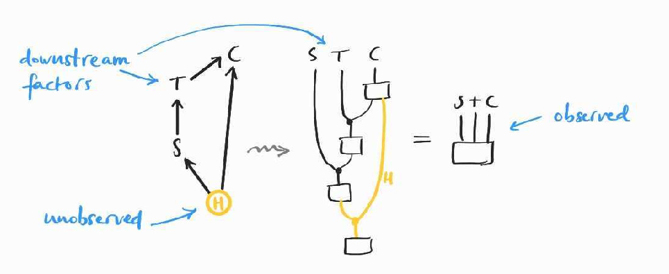
The key idea at this point is the following: while it is not clear how to compute the intervention at we already know how to compute interventions at , via the backdoor formula. To see this, notice that the models of the previous section and that of the new napkin problem have a similar structure if we squint enough, i.e. if we identify with , jointly with and with and jointly:
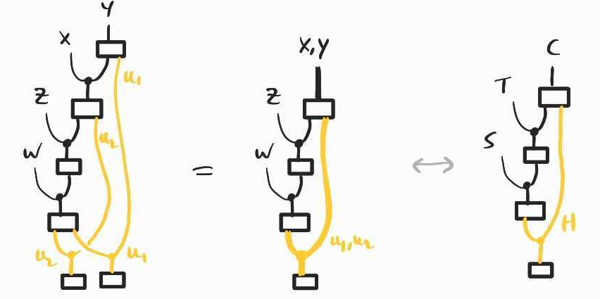
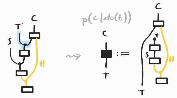
Thus, it is not difficult to see that interventions at in the new napkin problem follow the same pattern. In particular, we will care about (we will see why shortly). We can therefore apply the backdoor adjustment formula to this new model:
Why is this formula useful? We want to deduce what would happen if we intervened at and observed , from what would happen if we intervened at and observed and , because interventions at are easy to compute.
First, notice that if we intervene at then all confounders–the common causes and –for the causal effect of on are blocked. This explains why intervening at is helpful: given that we intervene at (and therefore block all confounders for the causal effect of on ), the causal effect of on can be estimated from observational data. In other words, we claim that intervening at and and observing is the same thing as intervening at and observing , conditional on . In do-notation, . And the latter can be estimated from , which we already have as .
Another way to get to same intuition is to notice that if we take the diagram for and compose it with , we get that of . This suggests the following derivation:
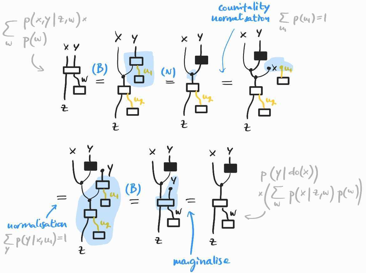
In the end, we have shown that . If is invertible (and in causal inference, we assume positivity of the probabilities involved most of the time), we can conclude that
There we have it: a probabilistic solution of Pearl's new napkin problem.
What next?
There is more to causal inference than causal identifiability. As I have been meaning to keep climbing Pearl's ladder of causation, I might cover counterfactuals in a subsequent blog post. As far as I know, anyone has yet to write about counterfactuals from the diagrammatic point of view. Stay tuned.
EDIT (27/05/23). Robin Lorenz and Sean Tull just released an arXiv preprint on causal inference with string diagrams, including a treatment of identifiability, counterfactuals and much more... Go check it out!