Basic causal inference via string diagrams

Does smoking cigarettes cause lung cancer? More precisely, what is the average causal effect of smoking cigarettes (say, for a decade) on contracting lung cancer? By now, this question has become the hello world of causal inference blog posts and introductions.

Causal inference proposes different ways of answering the question, under different assumptions. I will explore three of them using string diagrams for Markov categories and some extra axioms that I'll clarify along the way.

First, a bit of notation: following standard practice, I will write $p(c|do(s))$ for the average causal effect of smoking on cancer (we will define it more precisely below). I use capital letters $X,Y...$ for variables and lower case letters $x,y...$ for their values. Moreover, in all the diagrams below, empty boxes with variables $X_1, ..., X_n$ at the bottom and $Y_1,..., Y_m$ at the top represent the joint conditional $p(y_1,..., y_m|x_1,...,x_n)$. In other words, they are diagrams in the symmetric monoidal category of (finite) sets and stochastic maps between them, with the monoidal product given by the cartesian product. Because we work over a fixed sample space, we do not need to annote the boxes; they are all uniquely determined by their type. For more on how string diagrams can provide a nice axiomatic framework in which to rederive fundamental results of probability theory, I recommend having a look at Tobias Fritz' paper A synthetic approach to Markov kernels, conditional independence and theorems on sufficient statistics.

A non-answer

By now, everyone knows that correlation does not imply causation. Therefore, what we cannot do–at least in the absence of further assumptions–is say that the average causal effect of smoking on cancer is simply the conditional $p(c|s)$, obtained from observational data, i.e. from the joint distribution $p(s,c)$ observed in the population of interest. In the context of our example, there might be confounding factors that influence both relevant variables ($S$ and $C$, here) so that a smoker might be more likely to contract cancer for other reasons (genetic, cultural...).

RCTs: intervening on the cause

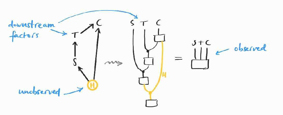
So what can we say about $p(c|do(s))$ in the presence of confounders? To say anything meaningful, we need to make our assumptions clear about the causal structure we think produces the data we observe. We can summarise the previous discussion with the following causal structure–where we call $H$ the confounding variables collectively–expressed in graphical terms and as an equation between string diagrams:

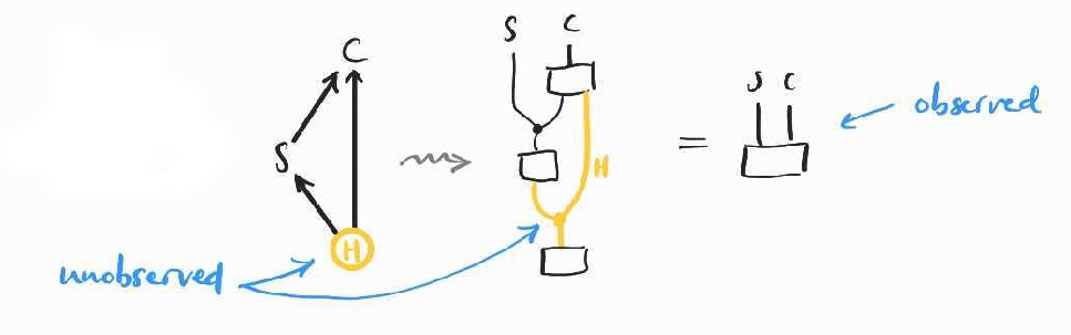
(This way of translating causal networks–which are just directed acyclic graphs btw–to string diagrams in Markov categories was first proposed by Brendan Fong in his masters' thesis.)

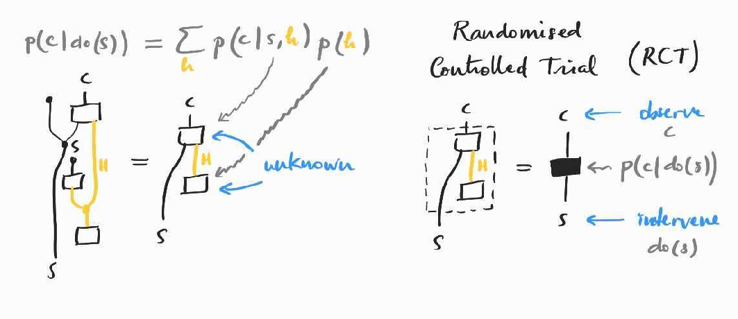
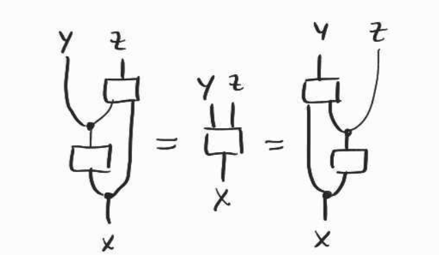
How is $p(c|do(s))$ even defined? Brushing aside many philosophical issues, we define the average causal effect $p(y|do(x))$ as the probability of observing $Y=y$ if we intervene at $X$ to set it to the value $x$. In the absence of parallel universes, the standard way of computing this distribution is by running a randomised controlled trial (RCT) where we split the population into different subpopulations evenly and set $X$ to one possible value for each subpopulation, and observe the outcome of $Y$. Going back to our example, to measure the causal effect of smoking on cancer, we would thus need to gather a random group of people, select half randomly and force them to smoke for a few decades (while making sure the other half does not smoke). At the end of the trial, we can simply count how many in each group have contracted lung cancer to obtain $p(c|do(s))$ and $p(c|do(\lnot s))$. Diagrammatically, this amounts to severing the wire for $S$ and extending it to the bottom as on the left below (and discarding all top wires we no longer need):

(A similar idea appears in a paper by Jacobs, Kissinger and Zanasi if you want to see where I'm taking that from. )

We will see below (in the context of the second method) how we derive the simpler form of $p(c|do(s))$. It is not so important here because the simplified string diagram still contains some unobservable quantities (those that depend on $H$), so we cannot compute it from observational data. The only way to reliably estimate the interventional probability $p(c|do(s))$ in this case is by running the trial itself. The diagram also illustrates how $p(c|do(s))$, denoted by the black box on the right, is in general not $p(c|s)$.

While rigorous, RCTs cannot and should not always be carried out (as the smoking example makes clear)! Luckily, under different assumptions, there are other ways of estimating $p(c|do(s))$from observational data only.

Backdoor criterion: conditioning on all confounders

There is a first simple alternative, if we can list and observe all confounding variables. In this case, we can gather observational data for the joint $p(s,c,h)$, which allows us to control for the effect of $H$ and eventually compute $p(c|do(s))$.

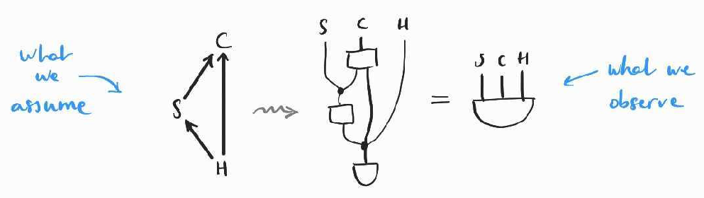
In practice, this amounts to subdividing the data into different subpopulations, for each possible value of $H$. The corresponding diagrammatic reasoning follows the same idea:

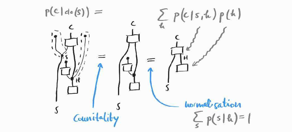
The formula we have derived is referred to as the backdoor adjustment:

Note that here we have only used the defining axioms of Markov categories: the counitality of the comonoid structure we assume we have, and the so-called causality axiom (which encodes the normalisation of probability distributions).

Frontdoor criterion: God's intervention via mediating factors

The real world is often messy and we can rarely identify all confounding factors for the causal effect we wish to estimate. One of the key insights of causal inference was that in some cases, if we can observe some mediating factors that sit in between our variables of interest, we are able to estimate the relevant causal effect from observational data. In the case of smoking, we could assume that tar deposits in the lungs ($T$) are a good proxy for the causal effect of smoking on cancer. For this third method to work, we need to also assume that $T$ is independent of the hidden confounders $H$ given $S$, and that it fully explains the causal influence of $S$ on $C$. Diagrammatically, this translates to:

Assuming the causal structure above, we can estimate the outcome of a RCT and compute the desired causal effect. Before showing how, we will need to assume a little more than the axioms of Markov categories.

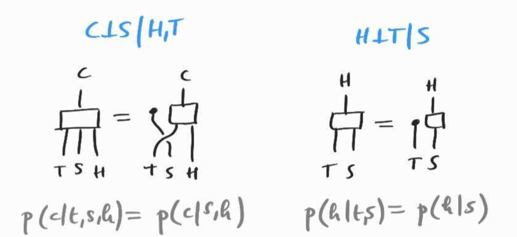
• First, we need to assume that our categories admits conditionals–we can find the relevant diagrammatic translation in the work of Tobias Fritz for example:

• Second, we assume the diagrammatic versions of the conditional independence equations that are compatible with the chosen causal model. Any causal model specifies some conditional independence conditions: concretely, every variable is independent of its non-descendants given its parents. For example, with the causal structure above, $T$ is independent of $H$ given $S$, and $C$ is independent of $S$ given $H$ and $T$, two facts which are usually written $T\bot H | S$ and $C\bot S | H,T$. Furthermore since independence is symmetric, we also have $H\bot T | S$. In the calculus of probability, these manifest as, e.g., $p(c|t,s,h)=p(c|s,h)$ and $p(h|t,s)=p(h|s)$. There are several ways of translating these facts in the context of Markov categories; here is one way that we will reuse later:

Now we are ready to compute $p(c|do(s))$. The challenge is in obtaining quantities that do not involve any unobserved variable ($H$ here). Diagrammatically, we attempt to remove all boxes with a yellow wire. We can do so as follows, using the axioms we have so far:

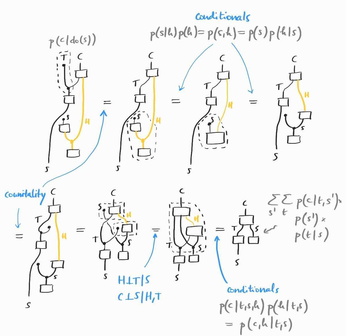
The formula we have rederived is commonly called the frontdoor adjustment formula:

[Added on 03/02/23: after reading Chapter 3 of Judea Pearl's Causality textbook, I have realised that the author gives the same derivation or, rather, that the derivation above is a diagrammatic translation of the one he gave. This makes sense, as we're not using any do-calculus, but only basic axioms of conditional probability and independence assumptions.]

One important point: we need the dependence of $T$ on $S$ to be noisy, that is, we want $p(t,s)$ to be positive for all $t$ and $s$. If, for example, $S=T$, then we could not compute the conditional $p(c|t,s)$ as values for which $T$ and $S$ differ have probability zero. In more conceptual terms, $T$ does not provide any additional information so we are back in the first scenario above, and would have to perform a randomised experiment to estimate $p(c|do(s))$.

The do-calculus and further work

How far can we push the ideas of this post? Could we give a fully diagrammatic and fully equational treatment of Pearl's do-calculus? In its original formulation, the do-calculus is given by three rules (in addition to the usual rules of probability theory) in the form of equations which can only be applied when the variables involved satisfy certain conditional independence conditions, read from particular dags (themselves derived from the assumed causal model). Therefore, if this is at all possible, one of the benefits of turning the do-calculus into equational reasoning over string diagrams, would be to dispense with the side-conditions and obtain a purely algebraic way of identifying causal effects. Since the conditional independence structure is baked into the diagrams, this is not an unreasonable hope.

In the epilogue of his book, Causality, Judea Pearl writes that "intervention amounts to a surgery on equations (guided by a diagram) and causation means predicting the consequences of such a surgery". We'd be aiming for a causal calculus that blends the usual two aspects of causal inference–-graphs and equations–-into a single diagrammatic formalism.

Inspired by our computations above, we could take as syntax the free Markov category over a set of generators quotiented by the equations imposed by the assumed causal model; in other words, we would throw in equations that encode the conditional independence of a variable on its non-descendants, given its parents. Which equations we need specifically remains to be seen given that, in a general Markov category, there are several inequivalent ways to represent conditional independence (I can think of at least two that we would need to encode $X\bot Y|W$, namely the diagrammatic versions of $p(x|yw)= p(x|w)$ and $p(xy|w)=p(x|w)p(y|w)$). I would also assume that we need a rule to express the existence of conditionals. With the right set up, we'd hope for the following...

Conjecture. All causal effects can be identified equationally in this category, i.e. it is complete for causal inference in the same sense that the do-calculus is complete: for variables $X,Y,Z$, the quantity $p(y|do(x),w)$ can be computed from observational data when we can rewrite the corresponding diagram (built from the dag generators as explained above or in e.g., Jacobs, Kissinger, and Zanasi's paper cited below) as a diagram containing only known quantities, using only the axioms of the previous paragraph.

References

• The structure of this post follows that of Marcus Lewis's Some "causal inference" intuition. The title is not a misnomer–-I found his post very helpful to build intuition about the frontdoor adjustment in particular.

• As I have already mentioned, the idea of turning causal networks into string diagrams is due to Brendan Fong; more details can be found in his masters' thesis Causal Theories: A Categorical Perspective on Bayesian Networks.

• The first treatment of interventional probabilities as string diagrams is due to Bart Jacobs, Aleks Kissinger and my coauthor, Fabio Zanasi in their paper Causal Inference by String Diagram Surgery. They treat the same example and give a criterion for causal identifiability in the diagrammatic representation of a given causal model. This is different from the equational approach I have followed here.

• Tobias Fritz's work on the synthetic approach to probability theory in Markov categories is really inspiring. I've referred to the treatment of conditionals in A synthetic approach to Markov kernels, conditional independence and theorems on sufficient statistics in Section 11 (in particular Definition 11.5) here, but the whole paper is well worth reading!

• Judea Pearl's textbook Causality seems to be the standard reference on causal inference; I have only read the epilogue, which is a leasurly introduction to the topic, and a shorter read than The Book of Why.