String diagrams for the \(\lambda\)-calculus?
Recently, on twitter, Davidad re-discovered a well-known graphical representation for terms of the \(\lambda\)-calculus, sometimes called sharing graphs or interaction nets. These graphical encodings have been the object of intense research for a long time. While it's not my area, I replied with a few tweets explaining some of the trade-offs of this approach as I saw it–from afar, admittedly. I concluded warning that these graphs are not usually understood as string diagrams, even if it is a natural question to ask: can we find a symmetric monoidal category for which they are genuine string diagrams? Crucially, can we do so in a way that respects the dynamic aspects of the \(\lambda\)-calculus, i.e. such that the graph-rewriting rules implementing \(\beta\)-reduction are valid equations in the underlying category?
This post gives one partial answer to this question. I will interpret diagrams as certain relations and show that \(\beta\)-reduction corresponds to inclusion of relations. The chosen semantics has the additional benefit of highlighting some of the issues that arise with copying/sharing of subterms during reduction. But before we get started, a word of warning: it is entirely possible that I am reinventing the wheel and I would love for someone to point me to the relevant papers if that is the case! (The syntactic part of this post is certainly not new, but the specific categorical semantics might be.)
Prerequisites. In this note, I assume familiarity with string diagrams, monoidal categories, and basic facts about the \(\lambda\)-calculus. To brush up on the first topic, Peter Selinger's survey is a safe reference.
Relational profunctors
First, we need a symmetric monoidal category in which to interpret our diagrams. This will be the category of relational profunctors. While profunctors can be scary, relational profunctors are their friendlier, decategorified cousins. The category of relational profunctors has preordered sets as objects and monotone relations \(R\subseteq X\times Y\) as morphisms \(X\rightarrow Y\). A relation is monotone if whenever \((x,y)\in R\) and \(x'\leq x\), \(y \leq y'\) then \((x',y')\in R\). Composition in this category is the usual composition of binary relations, given by \(R;S = \{(x,z) \,:\, \exists y.\, (x,y)\in R \land (y,z)\in S\}\), which we write in diagrammatic order. The identity on a preorder is none other than the order relation itself!
With the usual product of preorders – the cartesian product of sets with the order on pairs given by \((x,y)\leq (x',y')\) iff \(x\leq x'\) and \(y\leq y'\) – this category is symmetric monoidal, with unit for the monoidal product the singleton set \(1\) with the only possible order. Great – we have a canvas on which to draw string diagrams. In fact, it is a particularly nice setting because relational profunctors form a compact closed category: each object \(X\) has a dual \(X^{op}\) with the same underlying set but the opposite ordering, and arrows
 \(: 1 \rightarrow X\times X^{op}\) given by \(\{(\bullet, (x',x)) : x\leq x'\}\)
and
 \(: X^{op}\times X\rightarrow 1\) given by \(\{((x,x'),\bullet) : x\leq x'\}\)
satisfying the following intuitive equations[1] :
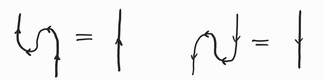
An upward flowing wire denotes (the identity on) \(X\), while a downward flowing wire denotes (the identity on) \(X^{op}\). The two equalities above relate an object to its dual and, diagrammatically, give us the ability to bend and straighten wires at will, as long as we preserve the overall directional flow[2] and the connectivity of the different components.
Application and abstraction as adjoints
In order to interpret our diagrams as relational profunctors, we first fix a single object – a preordered set \(X\) – equipped with a binary operation 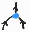 \(: X\times X \rightarrow X\). Note that we do not require that this relation be associative. You can think of \(X\) as a preordered set containing \(\Lambda\), the set of (closed) \(\lambda\)-terms ordered by the reflexive and transitive closure of \(\rightarrow_\beta\). In this particular case, you can take to be any monotone binary relation that restricts over \(\Lambda\) to (the graph of) application of \(\lambda\)-terms, \(\{((u,v),t) : uv \rightarrow^*_\beta t\}\). But we will prefer to work axiomatically, without committing to any specific model, simply requiring properties of \(X\) as we need them. In fact, one reason we do not simply take \(X=\Lambda\) is that we need our model to be better behaved than \(\Lambda\), so we enlarge it to get the desired properties. I'll come back to this point and give a construction of a suitable \(X\) and a possible interpretation later.
We chose to work with relational profunctors because we can also ask for the existence of adjoints where we need them.
Definition. (Adjunction for relational profunctors) We say that \(R: Y\rightarrow X\) is right adjoint to \(L: X\rightarrow Y\) iff
\[ id_X \subseteq L ; R \quad \text{and} \quad R ; L \subseteq id_Y \]where \(\subseteq\) denotes the inclusion of relations (seen as subsets).
To interpret abstraction we need a right adjoint to 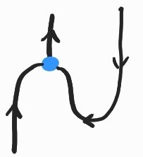 that we draw as
 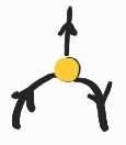 . Where does the adjunction come from? We can just postulate it as an axiom or, in the concrete example where \(\Lambda \subseteq X\) above, we can also ask that \(X\) be a complete (semi-)lattice; then, if also preserves joins in both arguments, we can define as \(\{((v,u),t) : v/u \leq t\}\) with \(v/u\) given by \(\bigvee\{t : tu \leq v\}\). Intuitively, for terms \(u\) and \(v\), this is the least upper bound of all terms that reduce to \(v\), when applied to \(u\). This may take us outside of \(\Lambda\) and this is why we need an \(X\) with a bit more leg room. The adjunction then follows from the equivalence \(tu\leq v \Leftrightarrow t\leq v/u\).
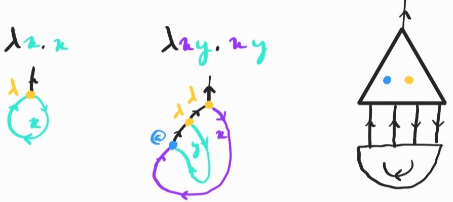
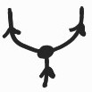
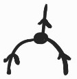
We now have enough machinery to encode linear \(\lambda\)-terms diagrammatically. By linear, I mean any term that uses each variable exactly once in its body. The translation is straightforward: linear terms are just trees of abstraction and application nodes, with at the bottom joining the wire indicating where a variable is applied to the wire indicating where it is captured by an abstraction:
All closed linear terms become arrows of type \(1\rightarrow X\) or, pictorially, diagrams with a single output wire at the top. We can translate open terms in the same way, leaving free variables as input wires at the bottom.
What about \(\beta\)-reduction? This is taken care of by one direction of the adjunction between and . Following (1), the first inclusion[3] becomes:
 or, equivalently,
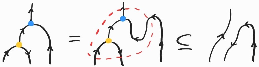
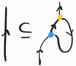
To see the connection with \(\beta\)-reduction more clearly, let's apply it to a redex of the form \((\lambda x.t)u\):
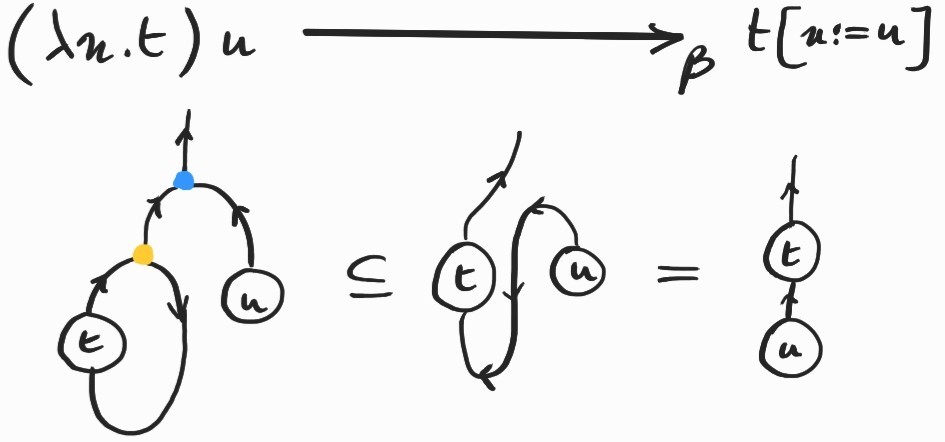
The at the bottom connects the wire representing the free \(x\) variable in \(t\) to the abstraction node. After applying the first inclusion, the \(x\)-wire gets reconnected to the argument, \(u\). The result is the diagrammatic counterpart of the substitution \(t[x:=u]\).
So far we've only used one side of (1). If the first inclusion corresponds to (linear) \(\beta\)-reduction, the second is \(\eta\)-expansion! Recall that it is given by \(t\rightarrow_\eta \lambda x. t x\) and it is not too hard to see that how this corresponds to the following inclusion:
I don't know if \(\eta\)-laws are a standard feature of the sharing graph/interaction net literature, but it certainly seems natural to include it here, as it constitutes one side of the adjunction between application and abstraction.
Copying and discarding
For any preorder, we also have a form of copying \(X \rightarrow X\times X\) given by
 \(=\{(t, (t_1, t_2)) : t \leq t_1 \text{ and } t ≤ t_2\}\).
For any preorder, we get a right adjoint to for free:
 \(= \{((t1, t2), t) : t1 \leq t \land t2 \leq t\}\).
Instantiating the two inclusions in (1), this means that
 \(\quad\) and \(\quad\)
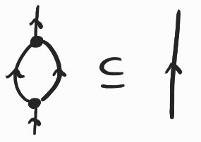
We need to discuss what happens when or interact with or .
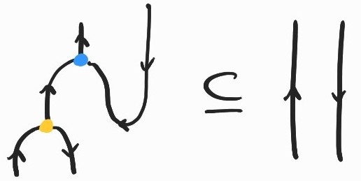
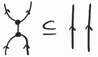
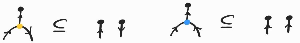
The point of introducing these last two generators was to duplicate certain diagrams. Luckily, the following inclusions always hold in our semantics, so that we can soundly duplicate or , as expected:
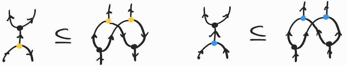
(The downward merge node is just whose bottom two wires are bent upward using two and whose top wire is bent downward using . We can always flip any arrow using the same idea.) Note that this is why we needed : when meets , we need some appropriate way of merging the two downward-flowing wires (corresponding to \(X^{op}\)) that result from this interaction, as in the inclusion on the left above.
Before drawing a few examples, there's one last component I have not mentioned yet: discarding. Sometimes we need to discard variables or entire subterms (to perform garbage collection in programming language slang). Technically, a discarding operation can be defined from what we already have as
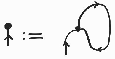
but it is more convenient to introduce a special generator in our syntax,  . Like our other generators, also has a right adjoint
  so that we have the following inclusions:
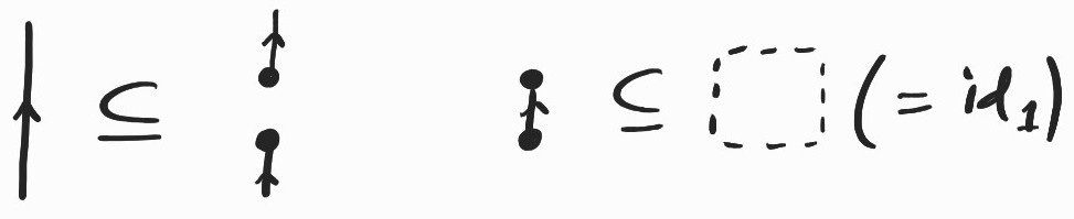
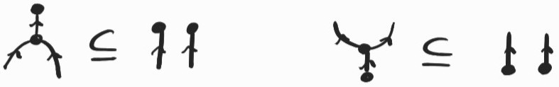
We can also delete or as the following inclusions hold:
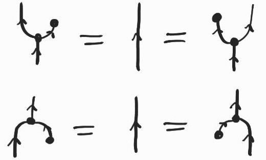
These new nodes also act as unit (resp. counit) for (resp. ):
Finally, and get duplicated when they meet and , respectively:
Putting it all together
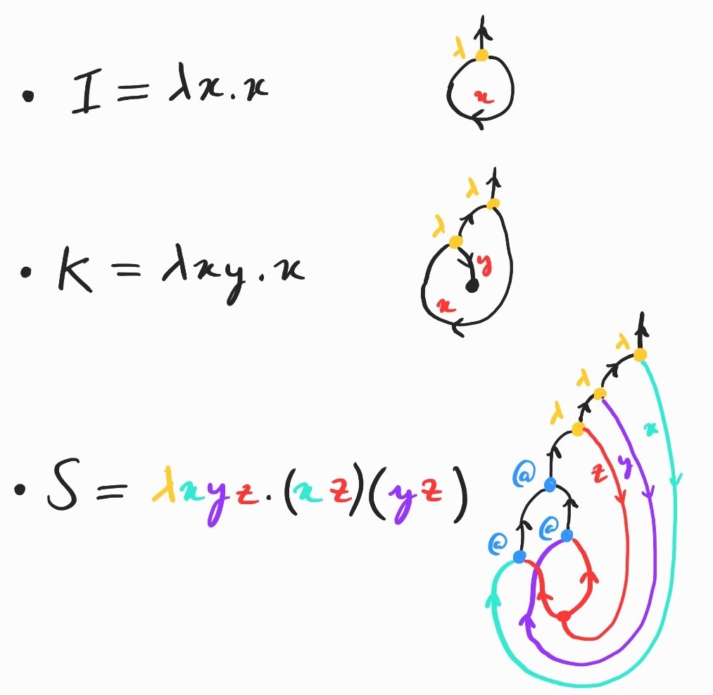
With copying and discarding, we can extend our encoding of linear \(\lambda\)-terms to all terms, simply copying a variable with when it is used multiple times or discarding it with when it is not used. Let's see it at work on a few standard examples:
The encoding of the static syntax is not the reason you read all this way, so let me show you how the diagrammatic counterpart of reduction behaves. All the inclusions we have covered so far can be interpreted as rewriting rules. The hope is that the resulting rewriting system is a diagrammatic implementation of \(\beta\)-reduction. As we will see, our wishes do come true sometimes, but not always.
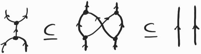
It is a basic exercise to show \(SKK\rightarrow_\beta I\). Here's how we can prove the same fact diagrammatically:
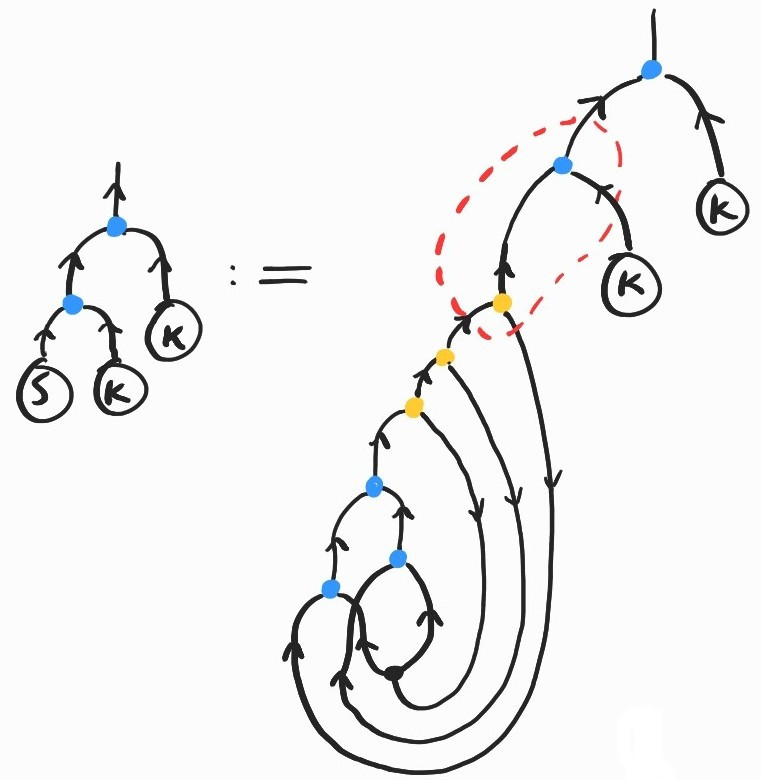
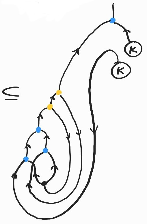
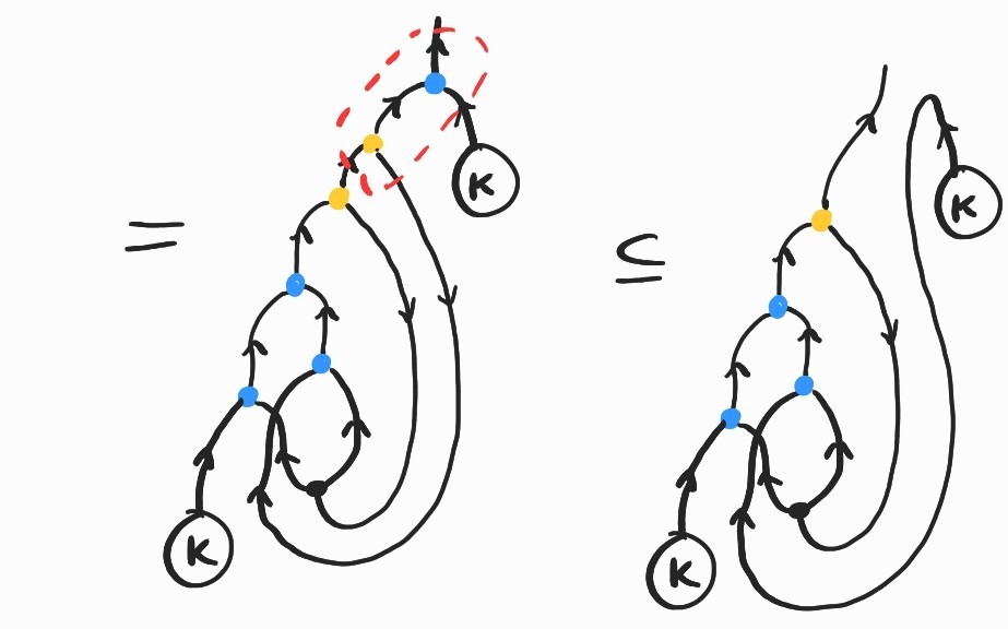
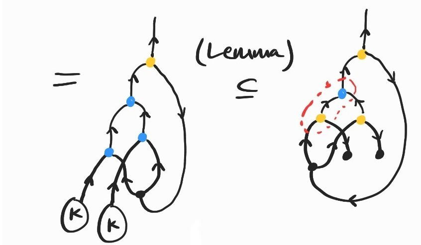
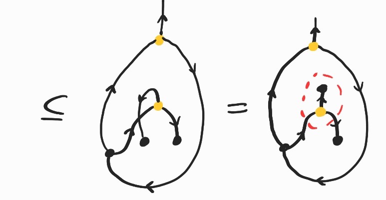
where the inclusion labeled (Lemma) comes from replacing \(K\) by its definition and applying the following twice:
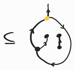
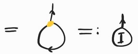
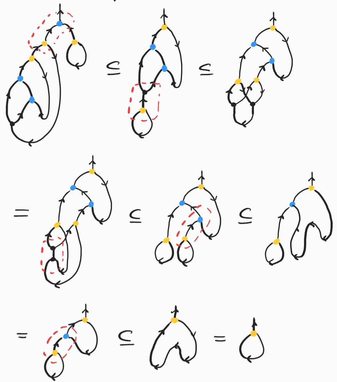
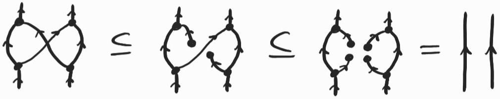
We have not yet used the adjunction between and , so let's compute another (useless) example: \((\lambda fx. f (f x)) (\lambda x.x)\). This amounts to applying the identity twice to an argument–-this should give us back the identity! Let's check that this is the case. This time I'll go a bit faster, but watch out for the third inclusion, where and cancel each other out:
Phew! If these examples seem long an tedious that's because they are. Not that it's fun to compute normal forms in the standard \(\lambda\)-calculus, but the diagrammatic version looks even more complicated. There is a good reason for this: one of the main points of graphical encodings of the \(\lambda\)-calculus is to make substitution explicit, operating at a finer level of granularity in order to keep track of resources more precisely. The thing is, on its own, the \(\lambda\)-calculus is too abstract to constitute a concrete model of computation; substitution, the engine of computation, is left as a meta operation. Even with a fixed reduction strategy (say, call-by-value) a single \(\beta\)-reduction step requires a global substitution of an argument for all occurrences of a bound variable inside the body of a term. This substitution cannot be implemented in constant time in general on a concrete model of computation, like a Turing machine or your actual physical computer. On the other hand, if you take a closer look at the diagrams above, you'll notice that, at each step, we only perform local rewrites, operating in constant time and space. Another advantage is that non-overlapping rewrites can be performed in parallel.
So what's the catch?
Well, unfortunately the naive procedure we've been using is not a refinement of \(\beta\)-reduction. The issue lies with the interaction of and .
The problem with copying
While we stay within the safe haven of the linear \(\lambda\)-calculus, the diagrammatic reduction procedure behaves exactly as its symbolic counterpart. But when we introduce copying, things get a lot more complicated: the inclusions from the two adjunctions above do not behave as \(\beta\)-reduction in general.
To understand the problem, notice that, in our strategy so far, if there are several occurrences of \(x\) in \(t\), when we reduce the expression \((\lambda x.t) u\), we will copy \(u\) by duplicating each of its components progressively. This might include duplicating nodes, creating nodes that will need to be eliminated later when they encounter their counterparts. However, if the copied term \(u\) itself contains copying nodes, things can go wrong.
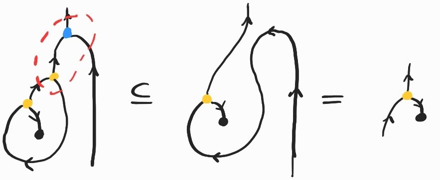
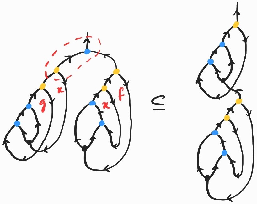
Let's see what the problem is on an example. Take \((\lambda x g. (g x) x)(\lambda f x. f (f x))\). Diagrammatically, the first few steps of the reduction process go as follows:
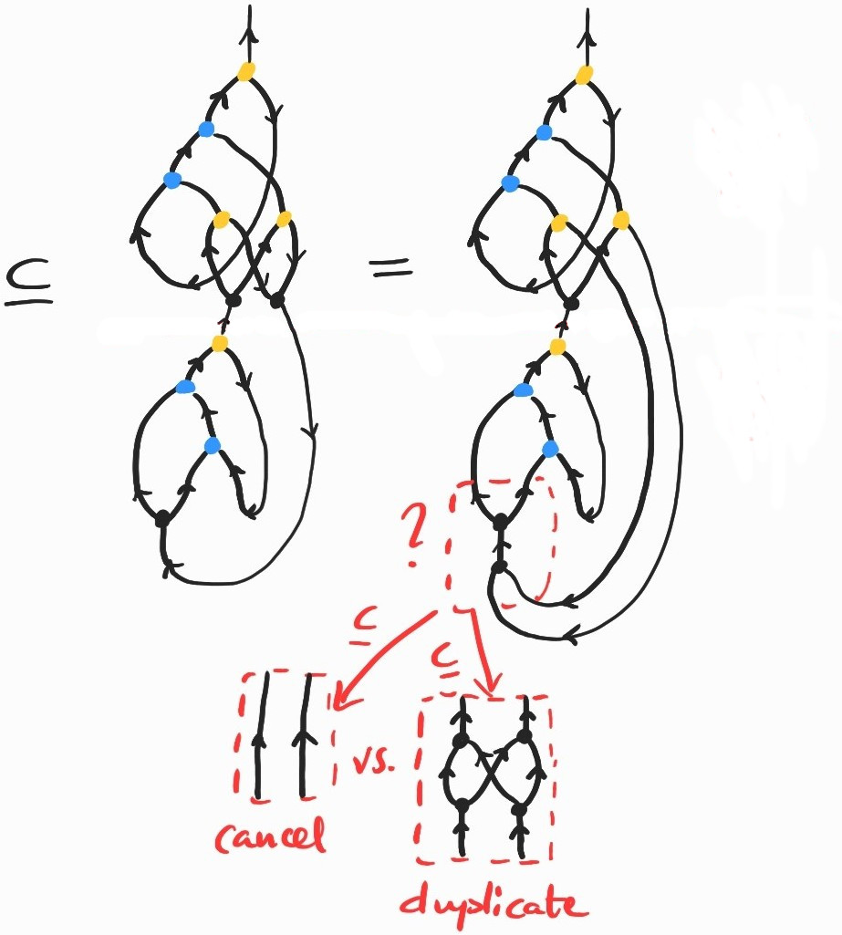
The last diagram illustrates the core of the issue: when the produced by copying the first abstraction node in \((\lambda x g. (g x) x)\) meets the copying node in the same term, they should duplicate each other instead of canceling out.
In summary, there are diagrams encoding well-formed \(\lambda\)-terms that we cannot copy. As I said earlier, this arises whenever we copy a term that itself contains a – in this case, those nodes generated by copying abstraction nodes should be duplicated when they meet nodes instead of the two canceling out. Diagrammatically, we would like:
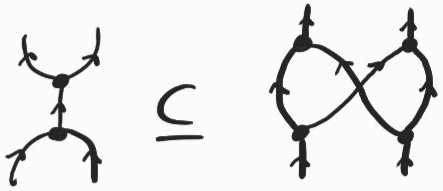
Not all is lost, however. Luckily for us, the corresponding inclusion holds in our chosen semantics. So where's the problem? We can just add it to our list of allowed rewrite rules and carry on our business as usual. Unfortunately, if we apply these inclusions haphazardly, two different choices may lead to different diagrams – how do we know which one is the right one?[4]
We now have to choose which rule to apply any time a meets a , following some specific strategy. This is a well-known problem in the literature on sharing graphs/interaction nets. There are different options to deal with it.
Some strategies involve keeping track of nesting of subterms. One way to do this is to introduce a notion of level and annotate nodes with the level at which they originate. Then, when
and from the same level interact, they cancel each other out, and when they belong to different levels, they duplicate each other. This requires a significant amount of bookkeeping. An equivalent implementation introduces global features, called boxes which enclose subterms, delimiting the level at which they live. Stefano Guerrini's gentle introduction to sharing graphs explains this. Alternatively, it is possible to determinise the rewriting strategy by keeping track of a token that moves around the graph and applies rewrite rules only where the token is located. This is the approach taken by François-Régis Sinot to encode call-by-value and call-by-need.
Another approach sidesteps the problem by disallowing terms that do not follow a form of syntactic stratification (if you're looking for the relevant keywords, they are terms typeable in elementary linear logic, a form of substructural logic with restricted copying, whose cut elimination procedure is guaranteed to terminate in elementary time in the size of terms).
A more radical approach is to accept that the correspondence between diagrams and terms is not perfect, and look for another syntactic encoding. What we have here is a Turing-complete graph rewriting system, so we are free to cook up any encoding of the \(\lambda\)-calculus we like, just like we could encode it on a Turing machine, register machine, or any other sufficiently expressive model of computation. Luckily, there are clever encodings that manage to stay close to the one we've seen here. For example, Ian Mackie and Jorge Sousa Pinto's translation, which reproduce features of the encoding of \(\lambda\)-terms as linear logic proofs[5], is not too difficult to understand.
Finally, a different approach is to bake hierarchical features into the syntax itself in order to capture higher-order functions explicitly. Davidad pointed out one way to do this (I was not aware of it prior to writing this post) which - I have since been told - solves the same problem: in this paper, Mario Alvarez-Picallo, Dan R. Ghica, David Sprunger, and Fabio Zanasi use hierarchical hypergraphs they call hypernets to encode the syntax of monoidal closed categories graphically (recall that the \(\lambda\)-calculus is also another syntax for cartesian closed categories).
Coming back to our string diagrammatic interpretation, one nice feature is that the problem with copying acquires semantic content. Let me explain. We have two different inclusions to deal with the composite ;. It turns out that these two possible choices can themselves be ordered:
This can be seen as a consequence of the adjunction between and :
In fact, it is not hard to construct \(X\) so that the first inclusion is an equality. So, if we always choose to duplicate and , we do not lose any semantic information. Of course, to recover a valid \(\lambda\)-term we will need to disconnect some wires eventually, using the second inclusion. This means that we can always postpone the choice of which wires to disconnect until the end. I found this surprising. Note that there is a space-time trade-off in this choice, as constantly duplicating nodes will increase the size of the diagram exponentially. In a way, we would be keeping track of all possible reductions, only committing to a specific form when disconnecting enough wires to recover a well-formed \(\lambda\)-term, i.e. a diagram made only from , , and . In order to do this we would also need to keep track of additional information in order to identify which wires to disconnect. I suspect that, by the conservation-of-work principle, we would need a mechanism at least equivalent to the different strategies I listed above.
What is \(X\)?
As we saw, if we can encode any \(\lambda\)-term as a string diagram, we can also draw diagrams that do not correspond to any term. In fact, some of these may appear during the reduction process, because diagrammatic reduction is more fined-grained than \(\beta\)-reduction. This is a feature and a bug, depending on how you look at it. A feature, because the point of introducing diagrams is to keep track of resources, via explicit copying and discarding. A bug, because the increased granularity needs to be approached carefully if we really want to mimic \(\beta\)-reduction.
To even draw these diagrams we needed our generators to satisfy certain properties. You may be wondering what these mean, semantically. Of course, you can approach the problem purely formally and say that these conditions are just what you need to implement \(\beta\)-reduction. But here's how I think about \(X\) in order to make all the required inclusions true. We can construct \(X\) as the set of downward-closed sets of \(\Lambda\). This is the free join semi-lattice over \(\Lambda\). Constructed in this way, the elements of \(X\) that are not principal, i.e. not of the form \(\{u\,: u\leq t\}\) for some term \(t\), can be thought of as generated by some set of terms. In other words, we can think of the elements of \(X\) as types! This might seem a bit strange because, from this point of view, terms are also types. But this is not so crazy if we view both types and terms as behaviours with varying degrees of nondeterminism. In other words, for two elements of \(X\), \(x\leq y\) can be read as \(x\) implements/refines/realises the specification \(y\). With this in mind, we can think of diagrams \(1\rightarrow X\) (with a single outgoing wire) that do not encode a \(\lambda\)-term as types or specifications that are not fully deterministic. I'm not entirely sure what this means, but it sounds profound.
References
Sharing Implementations of Graph Rewriting Systems, by Stefano Guerrini.
Call-by-Name and Call-by-Value as Token-Passing Interaction Nets, by François-Régis Sinot.
Compiling the lambda-calculus into Interaction Combinators, by Ian Mackie and Jorge Sousa Pinto.
Functorial String Diagrams for Reverse-Mode Automatic Differentiation, by Mario Alvarez-Picallo, Dan R. Ghica, David Sprunger, and Fabio Zanasi.
| [1] | Diagrams should be read flowing from bottom to top for composition, and from left to right for the monoidal product. |
| [2] | If you're already familiar with sharing graphs or interaction nets, you will notice that, unlike those, the edges of our diagrams are directed. Diagrams for relational profunctors can be drawn undirected iff \(X=X^{op}\) iff the underlying order is also symmetric, i.e. if it is the equality over \(X\). However, it is not clear in this case that abstraction can be defined over such an \(X\). Is this related to how there are no good set-theoretic models for the untyped \(\lambda\)-calculus and one needs to turn to more exotic constructions, like those of domain theory, for instance? Perhaps someone else can enlighten me here. |
| [3] | Usually, denotational semantics for the untyped \(\lambda\)-calculus require \(\beta\)-equal terms to have the same denotation. We only ask here for \(\beta\)-reduction to be interpreted as an inclusion. Perhaps we could modify our presentation to construct an \(X\) such that \(X\times X^{op} \cong X\), in order to obtain a more standard semantics. |
| [4] | I originally wanted to write that the resulting rewriting system was no longer confluent. While technically true, this is also the case of the previous system, if we include the use of inclusions coming from the adjunction between and . |
| [5] | The correspondence with linear logic is a recurring theme in this area. The boxes/levels I've mentioned are also a way of encoding the exponentials – the modality that controls access to copying and deleting in linear logic. |