The algebra of boolean satisfiability

They who are acquainted with the present state of the theory of Symbolical Algebra, are aware, that the validity of the processes of analysis does not depend upon the interpretation of the symbols which are employed, but solely upon the laws of their combination.

– The Mathematical Analysis of Logic, George Boole (1847)

Many roads lead to boolean satisfiability. In spite of its theoretical intractability and because of its surprising practical feasability, the problem has acquired a central importance in logic and computer science.

It is easy to state: given a Boolean formula $f$, does there exist an interpretation that satisfies $f$? In other words, it is the problem of determining if there exists an assignment of boolean values to the variables of $f$ that makes it true.

Boolean satisfiability, which we will just write as SAT from now on, is the paradigmatic NP-complete problem. Despite this theoretical barrier, SAT-solving has undergone a revolution in this millenium, with modern solvers now able to handle instances containing hundreds of thousands or even millions of literals.

What is there to say about SAT from an algebraic perspective? Surely everything has already been said a long time ago. George Boole worked out the algebraic laws of classical propositional logic in the 19th century. What new ideas could we possibly contribute here? Certainly, most of what I have writen below will look like a reformulation of old ideas, in a new language. But I am writing them here in the hope that others with similar interests find them useful and beautiful.

This post is a teaser for a preprint with Tao Gu and Fabio Zanasi. I am also grateful for many helpful discussions with Guillaume Boisseau's about the equational theory. (Actually, Guillaume has also started a Youtube channel on diagrammatic algebra, so go check it out!)

SAT is not algebraic

Let's start with a remark that will be obvious to many, but was not for me at first: SAT is not a problem that can be stated in the algebraic theory of boolean algebras. Let me explain.

An algebraic theory is a logical language in which we can form terms using variables and $n$-ary function symbols (including constants, which are just $0$-ary functions), and give axioms as equations between terms with free variables. A model of an algebraic theory is simply a set equipped with bona-fide functions of the appropriate arity interpreting each of the function symbols and satisfying the required axioms.

Thanks to Boole, we know that classical propositional logic can be formulated as an algebraic theory, whose models are what we now call boolean algebras.

There are several presentations of the algebraic theory of boolean algebras. One possible choice uses two binary function symbols $\lor,\land$ for disjunction and conjunction, one unary function symbol $\bar{\cdot}$ for negation, two constants $0,1$. The associated axioms are well-known and I won't list them all here. One example is that the conjunction of the same variable appearing twice, in positive and negative form, is equal to false:

$$x\land \bar{x} = 0$$

This is the algebraic counterpart of the propositional inference rule that allows us to derive a contradiction from... well, contradictory assumptions. Note that we can think of the free variables appearing in an axiom as implicitly universally quantified:

$$\forall x (x\land \bar{x} = 0)$$

This is because, in first-order logic, the two formulations make no difference in terms of what we can prove. Indeed, if we can prove a statement $P$ containing some free variable $x$ (meaning that we are not assuming anything about $x$), we can immediately derive a proof of $\forall x. P$. Conversely, if we have a proof of the $\forall x.P$, we can instantiate it by substituting any term into $x$.

There are many other presentations of the algebraic theory of boolean algebras: for example, it is well-known that a single binary function denoting NAND suffices (albeit with much less intuitive axioms). What matters is that the models of these different theories are all the same.

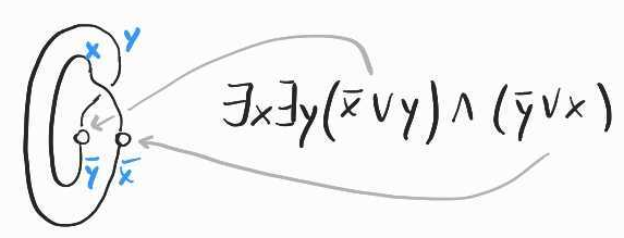
But wait – didn't I say that we are only allowed to use terms involving free variables for axioms? Satisfiability involves some existential quantifiers, so it is not clear how we could state it in an algebraic theory. This is what I meant when I wrote above that "SAT is not algebraic". Given a term $f$ in the theory of boolean algebras, containing free variables $x_1,\dots, x_n$, the logical statement that $f$ is satisfiable is

$$\exists x_1\dots\exists x_n (f = 1)$$

which is outside of the algebraic realm. It is not difficult to see that this statement is equivalent to

$$\lnot(\forall x_1\dots\forall x_n (\bar{f} =0))$$

The first-order formula $\forall x_1\dots\forall x_n \bar{f} =0$ can be seen as the equivalent unquantified statement $\bar{f} =0$ which is algebraic. So if we can prove $\bar{f} =0$, we know that $f$ is satisfiable. But if we cannot, this does not mean we have proven $\lnot(\forall x_1\dots\forall x_n \bar{f} =0)$. Not finding a proof of something is different from having a proof of its negation!

Boolean formulas have different canonical forms, with different use cases. For satisfiability, formulas are typically given in conjunctive normal form (CNF), i.e. as a conjunction of disjunctions of literals (variables or negated variables). The conjuncts are typically called clauses. The dual form disjunctive normal form (DNF) – a disjunction of conjunctions of literals – is trivial for satisfiability, since one can read all satisfying assignments of a DNF formula $f$ from its disjuncts directly. This suggests one way of dealing with SAT algebraically: use the axioms of boolean algebra to rewrite a CNF formula $f$ to DNF. In this form, each disjunct gives a satisfying assignment of the formula, and $f$ is satisfiable iff it has a non-contradictory term (one that does not contain $x\land\lnot x$. But this approach is not so useful if all we care about is satisfiability, as it requires computing all assignments in the process, potentially writing down a number of terms exponential in the size of the $f$.

We don't want to compute all satisfying assignments of a given $f$, we just care about the existence or non-existence of one. This is where the existential quantification comes in. It is what allows us to forget some information in the process of looking for such an assignment. Consider for example $f =(C\lor x)\land (\lnot x\lor D)$. Then $\exists x f = C\lor D$ since we don't really care about the value of $x$ anymore – $f$ is satisfiable iff $C\lor D$ is (this is an application of the important resolution rule. We'll come back to this below).

Hopefully this has convinced you that the algebraic theory of boolean algebras is not a convenient theory in which to encode SAT. Of course, we can just use a first-order existential statement to encode it, and use the full might of first-order logic to reason about SAT instances. But I'm looking for something that is more closely tailored to SAT itself, sufficiently expressive to encode the problem, but not much more. More importantly, I am looking for a genuinely algebraic treatment, in which simple equational axioms are sufficient to derive the (un)satisfiability of any given instance.

I will show below that an algebraic treatment of SAT is possible, if we are willing to move to a different syntax. Unsurprisingly, this syntax will be diagrammatic.

SAT is algebraic, diagrammatically

Why would we need a diagrammatic syntax? As we saw in the previous section, the algebraic theory of boolean algebras is insufficiently expressive. So we're looking for some other formal system.

Existential quantification is what gives SAT a particularly relational flavour: we are not simply evaluating boolean functions, but checking that there exists some assignment for which the function evaluates to true. This is a fundamentally relational, not functional constraint. In my experience, diagrammatic calculi are particularly well suited to express relational constraints. In fact, one way to think about string diagrams for relations is as a generalisation of standard algebraic syntax to the regular fragment of first-order logic, i.e. the fragment containing truth, conjunction, and existential quantification. In this setting, string diagrams have the advantage of highlighting key structural features, such as dependencies and connectivity between different sub-terms/diagrams.

We'll proceed in two steps. First I'll present a diagrammatic syntax to encode sets of boolean constraints before explaining how we can represent SAT instances in this language. Then, I will give a number of axioms that we can use to derive the (un)satisfiability of any given instance purely equationally.

A diagrammatic syntax for SAT

The language I'll introduce now is a graphical notation for managing sets of boolean constraints expressed in CNF.

A diagram with $n$ dangling wires at the top and $m$ at the bottom is interpreted as the set of satisfying assignments of some CNF formula over the set of variables $y_1,\dots,y_m,x_1,\dots,x_n$ (which we will see how to construct below). The constraint comes from setting the corresponding CNF formula to $1$. We will keep this implicit from now on, writing $(x_1\lor \bar x_2\lor x_3)\land (x_2\lor \bar x_1)$ instead of $(x_1\lor \bar x_2\lor x_3)\land (x_2\lor \bar x_1) = 1$. We will often use the CNF formula as a shorthand for its satisfying assignments, as it is a convenient notation for this set. But our diagrams are interpreted as sets though, if you prefer, you can also think of them as CNF formulas quotiented by the equivalence relation that identifies any two formulas that have the same satisfying assignments.

We have a few simple generating nodes, listed below.

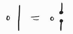
• A plain wire is used to encode an implication between two variables, $\bar y\lor x$:

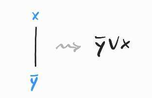
• A white node constrains the associated variables to satisfy $\bar y_1 \lor \dots\lor \bar y_n \lor x_1 \lor \dots \lor x_m$:

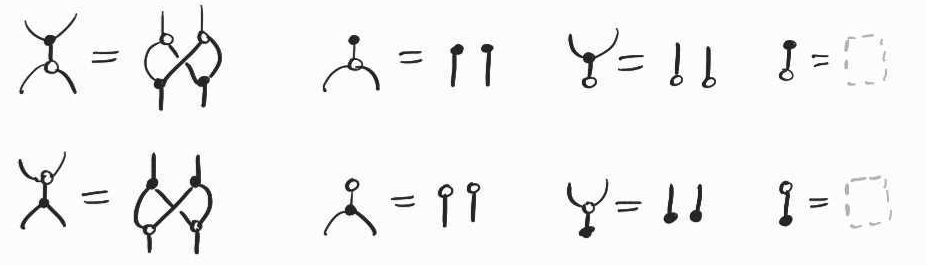
A few special cases. A white node with only one bottom leg and no top leg represents the constraint $\bar y_1$ (forces this variable to be false) and, conversely, a white node with a single top leg but no bottom leg, represents the constraint $x_1$ (which forces this variable to be true). A white node with no dangling wires at all is a contradiction, which has no satisfying assignment (and therefore represents the empty set).

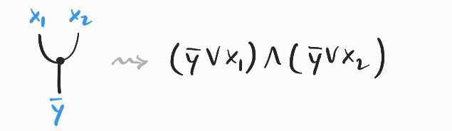
• A ternary black node with two bottom legs can be thought of as copying its top leg and enforces $(\bar y_1\lor x)\land (\bar y_2\lor x)$:

• Dually, a ternary black node with one bottom leg and two top legs is interpreted as $(\bar y \lor x_1)\land (\bar y \lor x_2)$:

• Unary black nodes places no constraints on their associated variable:

We also need to explain how to interpret composite diagrams.

Placing any two diagrams side by side (without connecting any of their wires) corresponds to taking the product of the two associated relations:

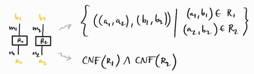
Here the $a_i$ and $b_i$ represent booleans that constitute the satisfying assignment of the corresponding formulas. At the level of formulas, the same operation corresponds to taking the conjunction two associated CNF formulas, which is still in CNF.

Things get a bit more interesting when we connect two wires. In general, we can connect several wires together in a single operation, which we depict as vertical composition and interpret as relational composition:

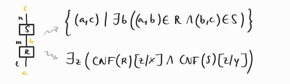
At the level of the formulas, this is interpreted by first identifying the two opposite literals that share the same wire, and existentially quantifying over this variable. In other words, if the semantics of the first diagram $c$ is given by a CNF formula of the form $C\land (C_1\lor x)\land\dots\land(C_k\lor x)$ where the $C_i$ are all the clauses in which the variable $x$ appears and the diagram $d$ is given by $D\land (D_1\lor y)\land\dots\land(D_l\lor y)$, where the $D_i$ are all the clauses in which the variable $y$ appears, then joining the $x$-wire and the $y$-wire, gives

$$\exist z(C\land (C_1\lor z)\land\dots\land(C_k\lor z)\land D\land (D_1\lor z)\land\dots\land(D_k\lor z))$$

with $z$ fresh to avoid capturing some other variable.

One last thing: we're allowed to cross wires as long as we preserve the connectivity of the different parts. This is just variable naming/managment.

Depicting SAT instances

Given these generators and the two rules to compose them, we can represent any SAT instance as a diagram. Before giving you the general procedure, let's see it at work on two simple examples.

The first is $\exist x\exist y(\bar x\lor y)\land (x\lor \bar y)$. Here, we have two variables that appear as negative and positive literals. So we will need two white nodes – one for $x,\bar x$ and one for $y,\bar y$, each with two bottom wires, to encode the relationship $x\lor \bar x$ and $y\lor \bar y$:

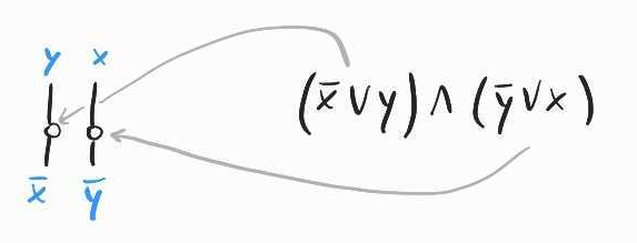
Each of these wires correspond to a literal that appears precisely once in one of the two clauses. We can just connect them directly to two white nodes representing each of the two clauses in $(\bar x\lor y)\land (x\lor \bar y)$. This gives:

For another example, let's consider the formula $\exist x\exist y(x\lor y)\land (\bar x\lor y)\land (x\lor \bar y)\land (\bar x\lor \bar y)$. Applying the same principle as above, we need two white nodes with two bottom wires each. We now have four clauses, so we will need four white nodes, each with two top wires for each of the variables appearing within the relevant clause:

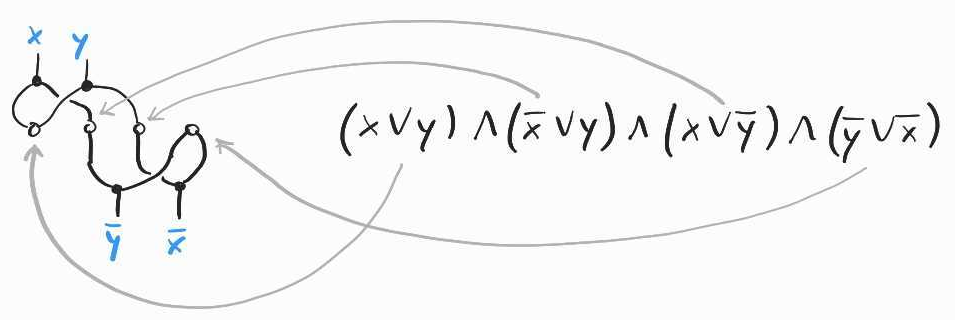
Each literal appears in two clauses, so we have more wires at the bottom of the diagram than at the top. To deal with this, we can simply duplicate each of the wires to connect the corresponding literal to the appropriate clause and get the diagram encoding the whole SAT instance. As before, we finish by connecting opposite literals at the top and at the bottom:

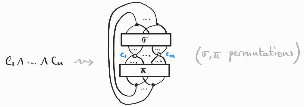
From these two examples, it is clear how one can use the same idea to encode arbitrary SAT instances. First, juxtapose as many white nodes with two bottom wires (and no top wires) as there are variables in the formula. Then, for each clause add a white node with as many top wires as it contains literals (and no bottom wires). Finally, connect the clauses to literals, duplicating or discarding wires where necessary. This takes the following form:

Monotonicity and negation. Some readers might have noticed something strange about our encoding of SAT: in the diagrammatic syntax, we can never enforce that a variable is the negation of another, as we do not have unrestricted access to a negation operation. Here, negation is a change of direction of a wire. This leads to an apparent mismatch between the diagrammatic and standard CNF representation of a SAT instance. A a variable appearing as a positive and negative literal in a given instance, appears as the bottom and top wire connected to some white nodes. The relationship between the two occurrences is given by the clause $\bar y\lor x$, for two different variables $y$ and $x$. This leaves the possibility of setting both variables to $0$, which satisfies $\bar y\lor x$ but does not match the intuition that these two variables should be negated version of each other. However, we can show that the assignment $y=1, x=0$ does not affect the satisfiability of the overall diagram representing the corresponding SAT instance. An issue can only arise if the assignment $y=1, x=0$ is required to make the diagram satisfiable. But this can never be the case because $y$ always appears negatively as $\bar y$ in any clause and $x$ always appear positively. This implies that the satisfiability of the clauses in which they appear will only depend on the other variables and therefore leave the overall unsatisfiability of the diagram unaffected.

Axioms for SAT

We don't just want to draw SAT instances as diagrams in this syntax; we would also like to reason about them directly at the level of the diagrams, without having to compile them to their CNF interpretation. In particular, we would like to derive the (un)satisfiability of a diagrammatic instance purely equationally, as we do when reasoning about standard algebraic syntax.

The axioms we'll need all take the form of equations between diagrams with potentially dangling wires. This is the diagrammatic counterpart of axioms between algebraic terms involving free variables. The difference is that a diagrammatic axiom can involve some composite diagram with wires that are not dangling. At the semantic leve, this allows us to specify equations that involve existentially quantified variables, when at the syntactic level we are reasoning purely equationally. This is where, in my opinion, lies the power of diagrammatic algebra (more on this in the additional remarks at the end of the post).

Some of these axioms can look daunting for the uninitiated. But, like for algebraic theories, there is a recurring cast of familiar characters that one learns to recognise. First of all, as I explained earlier, the diagrammatic syntax generalises the usual algebraic term syntax so, if you're familiar with the latter, you will recognise the usual suspects, like monoids, semirings, or rings, some commutative, some idempotent etc. Diagrammatic syntax also allows us to speak about dual operations, like co-monoids, that can cohabit(!) with their standard algebraic counterpart, and interact with them in different ways.

I'll introduce the cast progressively.

The black co-copying and co-discarding nodes form a monoid, while copying and discarding nodes together form a commutative comonoid. This means that they satisfy mirrored versions of the associativity, unitality and commutativity axioms of commutative monoids.

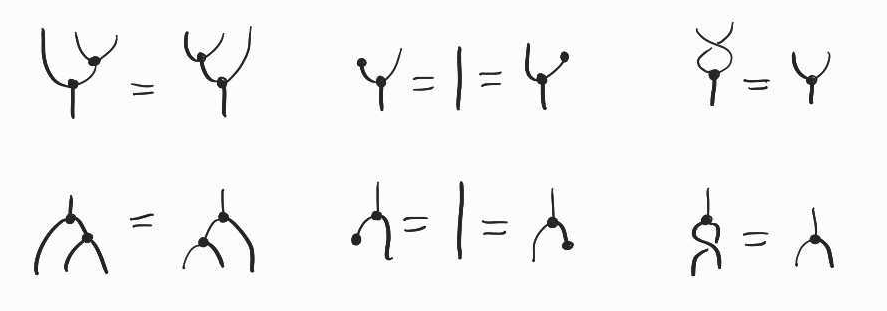
White nodes form what is called a commutative Frobenius algebra. This is a very convenient structure, which has a natural diagrammatic axiomatisation – every connected diagram of white nodes, can be collapsed to just a single node, keeping the dangling wires fixed:

This axiom is sound for our semantics because $\exists x.(C\lor x)\land (D\lor \bar x)$ is equivalent to $C\lor D$. It is thus the diagrammatic translation of the resolution rule in classical porpositional logic!

Notice that when we collapse several white nodes to a single one, we may introduce loops, if the original diagram is not simply connected:

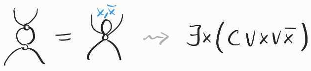
This is interpreted as $\exists x (C\lor x\lor \bar x)$ for some clause $C$. We can always satisfy $x\lor \bar x$ and therefore the whole clause $C\lor x\lor \bar x$, regardless of $C$'s value. Hence we can remove all constraints associated with $C$. Diagrammatically, this amounts to adding the following axioms:

Another worthy special case: when the network has no dangling wires, it represents a contradiction. For example,

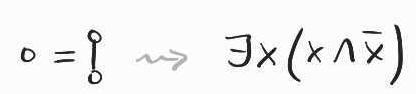
is interpreted as $\exists x(x\land \bar x)$, which is clearly contradictory. By the principle of explosion, a contradiction allows us to derive anything we want. Diagrammatically, this principle is translated as a rule that allows us to disconnect any wire:

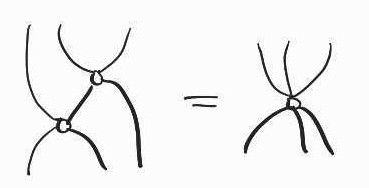
An important principle in logic is that conjunctions distribute over disjunctions. Even though our language deals with constraints in CNF, the distributivity of the underlying lattice is witnessed by the following laws that allows us to push white and black nodes past each other:

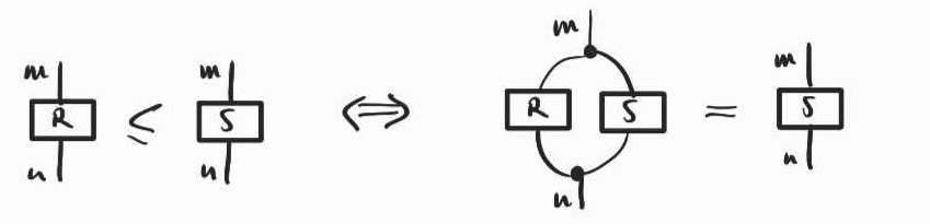
So far, I have only used equational axioms, but we also need some inequalities. Formally, the expressive power of our equational theory does not change by adding inequalities. In fact, the inequality relation can be defined using just equality and the black nodes:

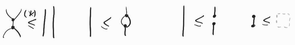
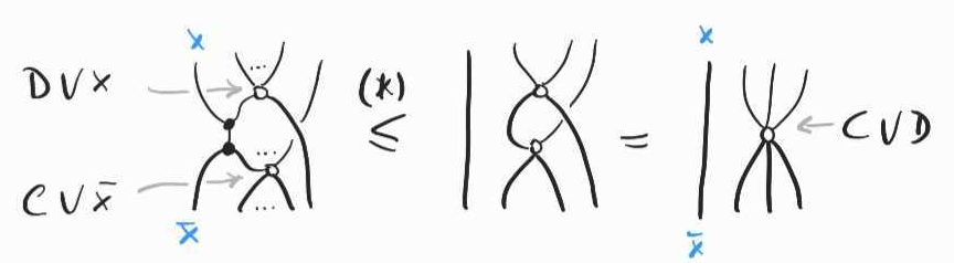
The following are important inequalities, that can be found in many other relational languages (they are the central axioms of a structure called a cartesian bicategory, which is what we have here):

Completeness. With Tao we have shown that with only a few more axioms, the equational theory complete for the given semantics in terms of boolean formulas. This means that if any two diagrams have the same semantics, we can show that they are equal using only these equations. In other words, you can forget about the semantics, and just reason diagrammatically! For the details, check out the paper. All I will say for the moment is that the completeness proof is reminiscent of quantifier elimination algorithms.

Additional remarks

SAT-solving in all this

One of the nice things about this language is that we can show that a given diagram represents a satisfiable instance or not by reasoning purely equationally at the level of the diagrams themselves. We treat the two examples above in the paper. The general strategy is very similar to heuristics that modern SAT solvers use.

Modern SAT solvers rely on Clause-Driven Conflict Learning (CDCL), itself an improved version of the Davis–Putnam–Logemann–Loveland (DPLL) algorithm. There is a known correspondence between these two algorithms and restricted classes of resolution proofs. The latter is easy to understand in the diagrammatic syntax. It procedes by progressively merging clauses that contain literals appearing in positive and negative form, until the diagram can be reduced to a single white node with no dangling wires, a contradiction (cf. above). This is perhaps best understood using inequalities, rather than the equalities of our axiomatisation.

Beyond standard SAT-solving heuristics, there is something potentially interesting about the algebraic approach I have sketched in this blog post: each axiom of our equational theory identifies rewrites for SAT instances that preserve the information we have about the instance. Contrast this with the naive approach to SAT-solving by computing every possible assignment. In doing so, for every value that we compute we learn some information that we then discard before computing a new value for the next assignment. In this process, some information is learned but immediately forgotten. The reason why modern SAT-solving algorithms, like DPLL and CDCL, generally work better than this brute force approach (though obviously not in the worst-case) is that, seen as resolution proofs, they learn new clauses at each step, and thus update their state of knowledge about the instance. Is it crazy to hope that, by identifying algebraic laws underlying deductions in SAT-solving, we will be able to explore different heuristics that are guaranteed to preserve the information we have already learned in the process of solving a given instance? Maybe.

But really, why a diagrammatic syntax?

An alternative to using string diagrams, is to move to an algebraic syntax with binders, as is often needed to model the syntax of programming languages with abstraction (e.g. the lambda calculus). Here, we would use the binders for existential quantifiers.

Terms of an algebraic syntax with binders can be seen as syntax trees with back pointers, so that the syntax is no longer one of labelled trees but of certain directed graphs. I would argue that the diagrams of this post are in fact a convenient notation for these graphs. The main difference is that, in our string diagrammatic syntax, the direction of the dangling wires enforces a type discipline that distinguishes positive and negative literals. Due to the monotonocity of our semantics, we do not have access to unrestricted negation, as I mentionned above. Neither do we have access to unrestricted existentital quantification – we can only existentially quantify pairs of opposite literals. This discipline is healthy, as it reduces the complexity of the diagrams and of the algebraic axioms (this is how we get the Frobenius law for example, which seriously simplifies the treatment of clauses).